Problem
C2.3. Analytical 3D
Body of Revolution
Overview
This problem is aimed at testing
high-order methods for the computation of external flow with a high-order curved
boundary representation in 3D. Inviscid, viscous (laminar) and turbulent flow
conditions will be simulated.
Governing
Equations
The governing equations for
inviscid and laminar flows are the 3D Euler and Navier-Stokes
equations with a constant ratio of specific heats of 1.4 and Prandtl number of 0.72. For the laminar flow problem, the
viscosity is assumed a constant.
Flow
Conditions
Inviscid:  Laminar:
  Turbulent:
Geometry
The geometry is a streamlined body based on a 10
percent thick airfoil with boundaries constructed by a surface of revolution.
The airfoil is constructed by an elliptical leading edge and straight lines.
Half
model:

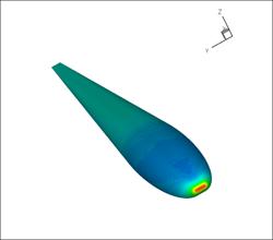
Figure 3D Body of Revolution
Reference values
Reference
area: 0.1 (full model)
Reference
moment length: 1.0
Moment
line: Quarter chord
Boundary
Conditions
Far field boundary: Subsonic
inflow and outflow
Wing surface: no slip
adiabatic wall
Requirements
1.
Start
the simulation from a uniform free stream everywhere, and monitor the L2
norm of the density residual. Track the work units needed to achieve steady
state. Compute the drag and lift coefficients cd and cl.
2.
Perform
grid and order refinement studies to find “converged” cd and cl values.
3.
Plot
the cd
and cl
errors vs. work units.
4.
Study
the numerical order of accuracy according to cd and cl
errors vs. ![]() .
.
5.
Submit
two sets of data to the workshop contact for this case
a)
cd and cl
error vs. work units
b)
cd and cl
error vs ![]()