Problem C2.4. Laminar Flow around a Delta Wing

Overview

A laminar flow at high angle of attack around a delta wing with a sharp leading edge and a blunt trailing edge. As the flow passes the leading edge it rolls up and creates a vortex together with a secondary vortex. The vortex system remains over a long distance behind the wing. This problem is aimed at testing high-order and adaptive methods for the computation of vortex dominated external flows. Note, that methods which show high-order on smooth solutions will show about 1^st order only on this test case because of reduced smoothness properties (e.g. at the sharp edges) of the flow solution. Finally, also h-adaptive, and hp-adaptive computations can be submitted for this test case.

Governing Equations

The governing equation is the 3D Navier-Stokes equations with a constant ratio of specific heats of 1.4 and Prandtl number of 0.72. The viscosity is assumed a constant.

Flow Conditions

Subsonic viscous flow with M_∞= 0.3, and α = 12.5°, Reynolds number (based on a mean cord length of 1) Re=4000.

Geometry

The geometry is a delta wing with a sloped and sharp leading edge and a blunt trailing edge. The geometry can be seen from Fig. 5 which shows the top, bottom and side view of the half model of the delta wing.

Half model:

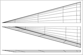
Figure 4: Left: Top, bottom and side view of the half model of the delta wing. The grid has been provided by NLR within the ADIGMA project. Right: Streamlines and Mach number isosurfaces of the flow solution over the left half of the wing and Mach number slices over the right half. The figures are taken from [LH10].

Reference values

Reference area: 0.133974596 (half model)

Reference moment length: 1.0

Moment line: Quarter chord

Boundary Conditions

Far field boundary: Subsonic inflow and outflow

Wing surface: no slip isothermal wall with .

Requirements

1. Start the simulation from a uniform free stream everywhere, and monitor the L₂ norm of the density residual. Track the work units needed to achieve steady state. Compute the drag and lift coefficients c_d and c_l.

2. Perform grid and order refinement studies to find “converged” c_d and c_l values.

3. Plot the c_d and c_l errors vs. work units.

4. Study the numerical order of accuracy according to c_d and c_l errors vs. . (Note, that due to the locally non-smooth solution, e.g. at the sharp edges, globally high-order methods will show about 1^st order only.)

5. Submit two sets of data to the workshop contact for this case

a) c_d and c_l error vs. work units

b) c_d and c_l error vs

6. The following data sets can also be submitted

a. for sequences of locally refined meshes (h-adaptive mesh refinement) and

b. for sequences of meshes with locally varying mesh size and order of convergence (hp-adaptive mesh refinement), possibly including improved data based on a posteriori error estimation results.

Note, that here the error-vs-work-unit data sets should take account of the additional work units possibly required

- for auxiliary problems (like e.g. adjoint problems),

- for the evaluation of refinement indicators or mesh metrics,

- and for the actual mesh refinement or mesh regeneration procedure.

References

[LH10] T. Leicht and R. Hartmann. Error estimation and anisotropic mesh refinement for 3d laminar aerodynamic flow simulations. J. Comput. Phys., 229(19), 7344-7360, 2010.