Problem C3.1. Turbulent Flow over a 2D Multi-Element Airfoil

Overview

This problem is aimed at testing high-order methods for a two-dimensional turbulent flow with a complex configuration. It has been investigated previously with low order methods as part of a NASA Langley workshop. The target quantity of interest is the lift and drag coefficients at one free-stream condition, as described below.

Governing Equations

The governing equation is the 2D Reynolds-averaged Navier-Stokes equations with a constant ratio of specific heats of 1.4 and Prandtl number of 0.71. The dynamic viscosity is also a constant. The choice of turbulence model is left up to the participants; recommended suggestions are 1) the Spalart Allmaras model, and 2) the Wilcox k-omega model.

Flow Conditions

Mach number M_∞ = 0.2, angle of attack α = 16^o, Reynolds number (based on the reference chord) Re = 9x10⁶. The boundary layer is assumed fully turbulent and no wind tunnel effects are to be modeled.

Geometry

The multi-element airfoil geometry is shown in the following figure. Originally the geometry is defined with a set of points. These points are then used to define a high-order geometry, which will be available online at the workshop web site.

The reference chord length is 0.5588 m.

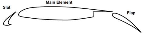
Figure 3.1. MDA 30P-30N multi-element airfoil geometry

Boundary Conditions

Adiabatic no-slip wall on the airfoil surface, free-stream at the farfield.

Grids

Participants may use their own grids for the convergence study. In this case, the geometry definition provided at the workshop web site should be used such that all the participants will use the same geometry. The workshop will also provide sample high-order computational meshes.

Requirements

1. Perform a convergence study of drag and lift coefficient, c_l and c_d, using one or more of the following three techniques:

a. Uniform mesh refinement of the coarsest mesh

b. Quasi-uniform refinement of the coarsest mesh, in which the meshes are not necessarily nested but in which the relative grid density throughout the domain is constant.

c. Adaptive refinement using an error indicator (e.g. output-based).

Record the degrees of freedom and work units for each data point, where the CPU t=0 corresponds to initialization with free-stream conditions on the coarsest mesh.

2. Submit two sets of data to the workshop contact for this case

a. c_l & c_d error versus work units

b. c_l & c_d error versus

Include a description of the coarsest mesh resolution and of the strategy used for refinement.